While each of us have our own list of favorite, most frequently used formulas, there is no standard list of top 10 formulas for everyone. So, today let me attempt that. If you want to become a data or business analyst then you must develop good understanding of Excel formulas become fluent in them. A good analyst should be familiar with below 10 formulas to begin with. To answer this question without the song and dance of excessive filtering selecting, you must learn SUMIFS formula. This magical formula can sum up a set of values that meet several conditions. The syntax of SUMIFS is like this: =SUMIFS( what you want to sumup, condition column 1, condition, condition column 2, condition….) Example: =SUMIFS(sales, regions, "A", products, "B", customer types, "C", month, "M") Learn more about SUMIFS formula. Pop quiz time …. Which of the below things would bring world to a grinding halt? A. Stop digging earth for more oil If you answered A or B, then its high time you removed your head from sand and saw the world. The answer is C (Well, if all coffee machines in the world unite miraculously malfunction that would make a mayhem. But thankfully that option is not there) The syntax for VLOOKUP is simple. =VLOOKUP(what you want to lookup, table, column from which you want the output, is your table sorted? ) Example: =VLOOKUP("C00023″, customers, 2, false) Lookup customer ID C00023 in the first column of customers table and return the value from 2nd column. Assume that customers table is not sorted. Click here to learn more about VLOOKUP Formula. Bonus: Comprehensive guide to lookup formulas. For every 10 people using VLOOKUP, there is someone realizing its most annoying limitation. VLOOKUP formula can only search on left most column. That means, if a table of customers has customer ID in left column and name in right column, when using VLOOKUP, you can search for customer ID only. You cannot ask questions like what is the customer ID of "Samuel Jackson" ? VLOOKUP would choke and bring your Excel world to a grinding halt. Thankfully, INDEX+MATCH formulas come to rescue. These 2 beautiful formulas help us lookup on any column and return corresponding value from any other column. Syntax: =INDEX(list of values, MATCH(what you want to lookup, lookup column, is your lookup column sorted?)) Example: =INDEX(customer IDs, MATCH("Samuel Jackson", Customer names, 0) ) Click here to learn more about INDEX MATCH formulas. Q: What do you call a business that does not make a single decision? A: Government! Jokes aside, every business needs to make decisions, even governments!!! So, how do we model these decisions in Excel. Using IF formulas of course. For example, lets say your company decides to give 10% pay hike to all people reading Chandoo.org 5% hike to rest. Now, how would you express this in Excel? Simple, we write =IF(employee reads Chandoo.org, "10% hike", "5% hike") The syntax of IF formula is simple: =IF (condition to test, output for TRUE, output for FALSE) Click here to learn more about IF formulas. Unfortunately, businesses do not make simple decisions. They always complicate things. I mean, have you ever read income tax rules?!? Your head starts spinning by the time you reach 2nd paragraph. To model such complex decisions situations, you need to nest formulas. Nesting refers to including one formula with in another formula. An example situation: Give 12% hike to employees who read Chandoo.org at least 3 days a week, Give 10% hike to those who read Chandoo.org at least once a week, for the rest give 5% hike. Excel Formula: =IF(number of times employee reads chandoo.org in a week >=3, "12% hike", IF( number of times employee reads chandoo.org in a week >0, "10% hike", "5% hike")) You see what we did above? We used IF formula inside another IF formula. This is nothing but nesting. You can nest any formula inside another formula almost any number of times. Nesting formulas helps us express complex business logic rules with ease. As an analyst, you must learn the art of nesting. Lots of nested formula examples explanations here. Most people jump in to Excel formulas without first learning various basic operators expressions. Fortunately, learning these requires very little time. Most of us have gone thru basic arithmetic expressions in school. Here is a summary if you were caught napping in Math 101. While there are more than two dozen text formulas in Excel including the mysterious BHATTEXT (which is used to convert numbers to Thai Bhats, apparently designed by Excel team so that they could order Thai take out food #), you do not need to learn all of them. By learning few very useful TEXT formulas, you can save a ton of time when cleaning data or extracting portions from mountains of text. As an aspiring analyst, at-least acquaint your self with below formulas: You can find several examples of all these formulas their users in our site. Just search. "There aren't enough days in the weekend" – Somebody Whether a weekend has enough days or not, as working analyst, you must cope with the working day calculations. For example, if a project takes 180 working days to complete and starts on 16th of January 2013, how would you find the end date? Thankfully, we do not have to invent a formula for this. Excel has something exactly for this. WORKDAY formula takes a start date working days and tells you what the end date would be. Like wise NETWORKDAYS formula tells us how many working days are there between any 2 given dates. Both these formulas accept a list of additional holidays to consider as well. More on working with Date Time values in Excel. Almost nobody asks about "Who was the second person to climb Mt. Everest, or walk on moon or finish 100 mtrs race the fastest?". And yet, all businesses ask questions like "Who is our 2nd most valuable customer?, third vendor from bottom on invoice delinquency? 4th famous coffee shop in Jamaica?" So as analysts our job is to answer these questions with out wasting too much time. That is where SMALL, LARGE formulas come in handy. Errors, lousy canteen food dysfunctional coffee machines are eternal truths of corporate life. While you can always brown bag your lunch bring a flask of finely brewed coffee to work, there is no escaping when your VLOOKUP #N/As. Or is there? Well, you can always use the lovely IFERROR formula to handle errors in your formulas. Syntax: IFERROR(formula, what to do in case of error) Use it like: IFERROR(VLOOKUP(….), "Value not found!") Click here to learn more about IFERROR Formula.1. SUMIFS Formula
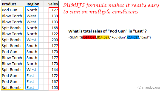 If you listen very carefully, you can hear thousands of managers around the world screaming… "How many x we did in region A, product B, customer type C in month M?" right now.
2. VLOOKUP Formula
B. Let US jump off the fiscal cliff or hit debt ceiling
C. Suddenly VLOOKUP formula stops working in all computers, world-wide, forever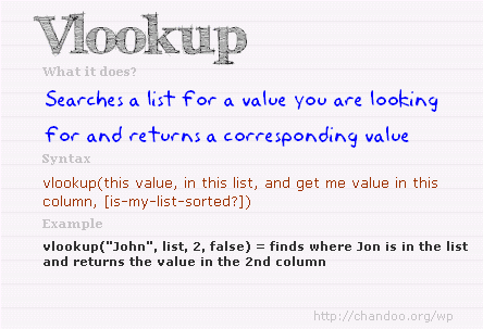 VLOOKUP formula lets you search for a value in a table and return a corresponding value. For example you can ask What is the name of the customer with ID=C00023 or How much is the product price for product code =p0089 and VLOOKUP would give you the answers.
3. INDEX+MATCH Formulas
4. IF Formula
5. Nesting Formulas
6. Basic Arithmetic Expressions
=(((123+456)*(789+987)) > ((123-456)/(789-987)))^3 " time I saw a tiger"
If you read the above expression and not had to scratch your head once, then you are on way to become an awesome analyst.
Operator What it does Example + – * / Basic arithmetic operators. Perform addition, subtraction, multiplication division 2+3, 7-2, 9*12, 108/3, 2+3*4-2 ^ Power of opetator. Raises something to the power of other value. 2^3, 9^0.5, PI()^2, EXP(1)^0.5 ( ) To define precedence in calculations. Anything included in paranthesis is calcuated first. (2+3)*(4+5) calcuates 2+3 first, then 4+5 and multiplies both results. To combine 2 text values "You are " "awesome" returns "You are awesome" % To divide with 100. 2/4% will give 50 as result. Note: (2/4)% will give 0.5% as result. : Used to specify ranges A1:B20 refers to the range from cell A1 to B20 $ To lock a reference column or row or both $A$1 refers to cell A1 all the time. $A1 refers to column A, relative row based on where you use it. For more refer to absolute vs. relative references in Excel. [ ] Used to structurally refer to columns in table ourSales[month] refers to the month column in the ourSales table. Works only in Excel 2007 or above. Know more about Excel Tables. @ Used to structurally refer to current row values in a table ourSales[@month] refers to current row's month value in oursales table. { } To specify an inline array of values {1,2,3,4,5} – refers to a the list of values 1,2,3,4,5 < > <= >= Comparison operators. Output will always be boolean – ie TRUE or FALSE. 2>3 will be FALSE. 99<101 will be TRUE. = <> Equality operators. Check whether 2 values are equal or not equal. Output will TRUE or FALSE 2=2, "hello"="hello", 4<>5 will all return TRUE. * ? Used as wild cards in certain formulas like COUNTIF etc. COUNTIF(A1:A10, "a*") counts the values in range A1:A10 starting with a. For more on this refer to COUNTIF SUMIF in Excel SPACE Intersection operator. Returns the range at intersection of 2 ranges A1:C4 B2:D5 refers to the intersection or range A1:C4 and B2:D5 and returns B2:C4. Caution: The output will be an array, so you must use it in another formula which takes arrays, like SUM, COUNT etc. 7. Text formulas
8. NETWORKDAYS WORKDAY Formulas

9. SMALL LARGE Formulas
10. IFERROR Formula
![]()
www.keralites.net 
![]()


| Reply via web post | Reply to sender | Reply to group | Start a New Topic | Messages in this topic (1) |
To subscribe send a mail to Keralites-subscribe@yahoogroups.com.
Send your posts to Keralites@yahoogroups.com.
Send your suggestions to Keralites-owner@yahoogroups.com.
To unsubscribe send a mail to Keralites-unsubscribe@yahoogroups.com.
Homepage: http://www.keralites.net
No comments:
Post a Comment